In [1]:
import matplotlib.pyplot as plt
import h5py
import numpy as np
import tensorflow as tf
from tensorflow.compat.v1 import ConfigProto
from tensorflow.compat.v1 import InteractiveSession

from PIL import Image
Image.MAX_IMAGE_PIXELS = None

from skimage.feature import match_template
import albumentations as A
import cv2
import os
import random

os.environ["CUDA_DEVICE_ORDER"]="PCI_BUS_ID"   # see issue #152
os.environ["CUDA_VISIBLE_DEVICES"]="0"

config = ConfigProto()
config.gpu_options.allow_growth = True
session = InteractiveSession(config=config)

TENSORBOARD_LOGDIR = 'moonlogs'

def get_images_and_masks(filename):
    with h5py.File(filename, "r") as f:
        # Divide by 255.0 to get floating point images.
        images = np.array(f['input_images'], dtype=np.float32) / 255.0
        masks = np.array(f['target_masks'], dtype=np.float32)
    return images, masks
In [2]:
transform = A.Compose([
A.HorizontalFlip(p=0.5),
A.VerticalFlip(p=0.5),
A.RandomRotate90(p=0.5),
A.GaussianBlur(p=0.2),
A.RandomBrightnessContrast(p=0.4),
A.ShiftScaleRotate(border_mode = cv2.BORDER_CONSTANT, p=0.5)
])
class MoonDataGenerator(tf.keras.utils.Sequence):
def __init__(self, inputs, outputs, batch_size = 16, augment = False):
self.inputs = inputs
self.outputs = outputs
self.batch_size = batch_size
self.augment = augment
num_samples, w, h = inputs.shape
self.inputs = self.inputs.reshape((num_samples, w, h, 1))
self.outputs = self.outputs.reshape((num_samples, w, h, 1))
def __len__(self):
"""Denotes the number of batches per epoch """
return len(self.inputs) // self.batch_size
def __getitem__(self, index):
batch_in = self.inputs[index*self.batch_size🙁index+1)*self.batch_size]
batch_out = self.outputs[index*self.batch_size🙁index+1)*self.batch_size]
if self.augment:
for i in range(self.batch_size):
inp = batch_in[i,...,0]
out = batch_out[i,...,0]
transformed = transform(image=inp, mask=out)
inp = transformed['image']
out = transformed['mask']
batch_in[i,...,0] = inp
batch_out[i,...,0] = out
return batch_in, batch_out
# Get the images and masks and shuffle them into a new train and test set.
train_images, train_masks = get_images_and_masks(filename = "train_images.hdf5")
dev_images, dev_masks = get_images_and_masks(filename = "dev_images.hdf5")
all_images = np.concatenate([train_images, dev_images])
all_masks = np.concatenate([train_masks, dev_masks])
total_images, _, _ = all_images.shape
shuffle = np.arange(total_images)
np.random.shuffle(shuffle)
all_images = all_images[shuffle, ...]
all_masks = all_masks[shuffle, ...]
# Create the generators for the neural network
TRAINING_DATA = int(0.8*total_images)
train_generator = MoonDataGenerator(all_images[:TRAINING_DATA], all_masks[:TRAINING_DATA], batch_size=64, augment=True)
dev_generator = MoonDataGenerator(all_images[TRAINING_DATA:], all_masks[TRAINING_DATA:], batch_size=8)
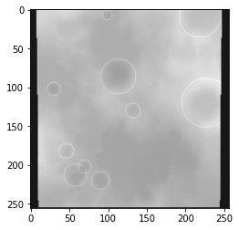
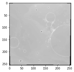
# Show some example images and their augmentations
for i in range(3):
inp, out = train_generator[i]
plt.imshow(inp[0,..., 0], cmap='gray', alpha=0.9)
plt.imshow(out[0,...], cmap='gray', alpha=0.1)
plt.show()

In [3]:
def unet(x, layers, num_output_channels):
    # Downsample
    x = tf.keras.layers.MaxPool2D(padding='same')(x)

    # Convolutions
    convolutions = layers[0]
    for num_neurons in convolutions:
        x = tf.keras.layers.Conv2D(num_neurons, 3, activation='relu', padding='same')(x)

    # Go deeper
    if len(layers) > 1:
        output_deeper = unet(x, layers[1:], convolutions[0])
        x = tf.keras.layers.Concatenate()([x, output_deeper])

    # More convolutions
    for num_neurons in convolutions:
        x = tf.keras.layers.Conv2D(num_neurons, 3, activation='relu', padding='same')(x)

    # Upsample
    x = tf.keras.layers.Conv2DTranspose(num_output_channels, 3, strides=2, padding='same')(x)
    return x

def build_model():
    x_in = tf.keras.layers.Input(shape=(None, None, 1))
    x = x_in

    for i in range(2):
        x = tf.keras.layers.Conv2D(32, 3, activation='relu', padding='same')(x)
    out_p1 = x

    x = unet(x, [[64, 64], [128, 128]], 32)

    x = tf.keras.layers.Concatenate()([out_p1, x])

    for i in range(2):
        x = tf.keras.layers.Conv2D(32, 3, activation='relu', padding='same')(x)
    output = tf.keras.layers.Conv2D(1, 3, activation='sigmoid',padding='same')(x)

    model = tf.keras.Model(inputs=x_in, outputs=output)
    return model

model = build_model()
model.summary()
model.compile(optimizer='adam', loss = tf.keras.losses.BinaryCrossentropy())
In [4]:
model.fit(train_generator,
          epochs=10,
          validation_data=dev_generator,
          callbacks=[
                  tf.keras.callbacks.TensorBoard(TENSORBOARD_LOGDIR+'/mymoondata',
                                                 update_freq='epoch',
                                                profile_batch=0,),  # log metrics
                ],)
model.save_weights('network.h5')
In [9]:
def predict_and_get_prediction_visualisation(image, model, draw_on_image = False):
"""
Code adapted from: https://github.com/silburt/DeepMoon/blob/master/utils/template_match_target.py
"""
w, h = image.shape
reshaped = image.reshape((1,w,h,1))
# Get the predicted semantic segmentation map
predicted_image = model(reshaped)
predicted_image = predicted_image[0,...,0]
# Settings for the template matching:
minrad = 2
maxrad = 100
longlat_thresh2 = 1.8
rad_thresh = 1.0
template_thresh = 0.5
target_thresh = 0.1
# thickness of rings for template match
thickness_ring = 2
target = np.copy(predicted_image)
# threshold the target
target[target >= target_thresh] = 1
target[target < target_thresh] = 0
coords = [] # coordinates extracted from template matching
corr = [] # correlation coefficient for coordinates set
for radius in np.arange(minrad, maxrad + 1, 1, dtype=int):
# template
size_template = 2 * (radius + thickness_ring + 1)
template = np.zeros((size_template, size_template))
cv2.circle(template, (radius + thickness_ring + 1, radius + thickness_ring + 1), radius, 1, thickness_ring)
# template match - result is nxn array of probabilities
result = match_template(target, template, pad_input=True)
index_r = np.where(result > template_thresh)
coords_r = np.asarray(list(zip(*index_r)))
corr_r = np.asarray(result[index_r])
# store x,y,r
if len(coords_r) > 0:
for c in coords_r:
coords.append([c[1], c[0], radius])
for l in corr_r:
corr.append(np.abs(l))
# remove duplicates from template matching at neighboring radii/locations
coords, corr = np.asarray(coords), np.asarray(corr)
i, N = 0, len(coords)
while i < N:
Long, Lat, Rad = coords.T
lo, la, radius = coords[i]
minr = np.minimum(radius, Rad)
dL = ((Long - lo)**2 + (Lat - la)**2) / minr**2
dR = abs(Rad - radius) / minr
index = (dR < rad_thresh) & (dL < longlat_thresh2)
if len(np.where(index == True)[0]) > 1:
# replace current coord with max match probability coord in
# duplicate list
coords_i = coords[np.where(index == True)]
corr_i = corr[np.where(index == True)]
coords[i] = coords_i[corr_i == np.max(corr_i)][0]
index[i] = False
coords = coords[np.where(index == False)]
N, i = len(coords), i + 1
# Get the raw prediction of only circles:
if draw_on_image:
target = image
else:
target = np.zeros(target.shape)
for x, y, radius in coords:
cv2.circle(target, (x,y), radius, (1.0,0,0))
return predicted_image, target
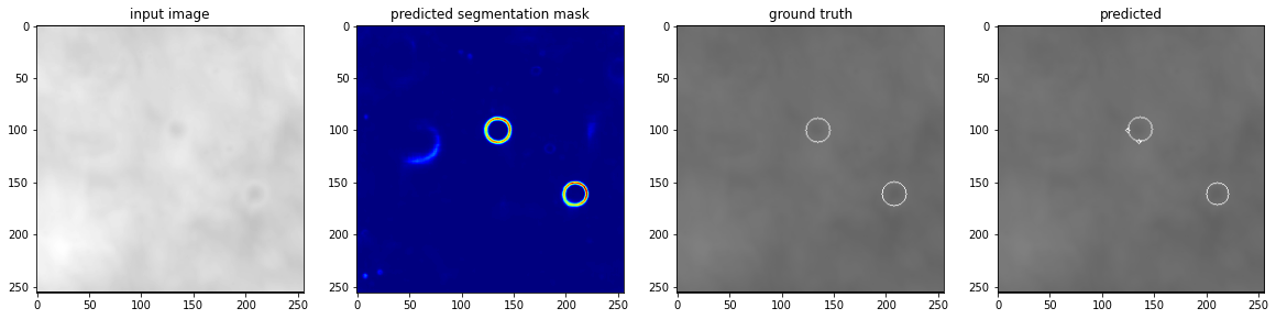
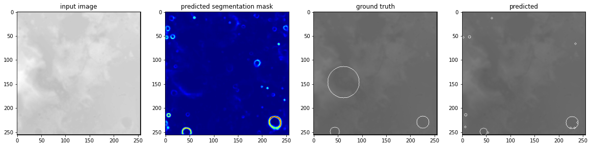
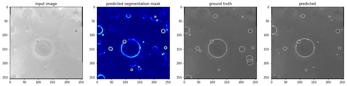
# For a few inputs, show both the input, segmentation mask, ground truth, and prediction.
for i in range(3):
inp, out = dev_generator[i]
first_image = inp[0,..., 0]
ground_truth = out[0,...,0]
predicted_segmentation, with_visualisation = predict_and_get_prediction_visualisation(first_image, model)
plt.figure(figsize=(20,20))
plt.subplot(141) # 1 row, 2 columns, Plot 1
plt.imshow(first_image, cmap='gray')
plt.title('input image')
plt.subplot(142)
plt.imshow(predicted_segmentation, cmap='jet')
plt.title('predicted segmentation mask')
plt.subplot(143)
plt.imshow(first_image, cmap='gray')
plt.imshow(ground_truth, cmap='gray', alpha=0.5)
plt.title('ground truth')
plt.subplot(144)
plt.imshow(first_image, cmap='gray')
plt.imshow(with_visualisation, cmap='gray', alpha=0.5)
plt.title('predicted')
plt.show()
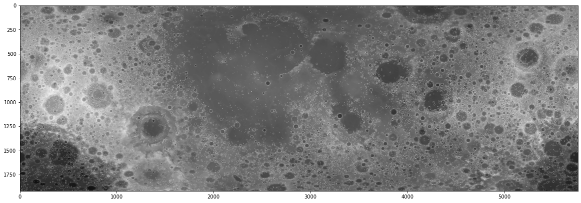
In [10]:
# Load the large image
im = Image.open("LunarLROLrocKaguya_118mperpix.png")

# Resize the image, because that is closes to the traiing data
w, h = im.size
raw_input_image = np.array(im.resize((w//16, h//16)))
w, h = raw_input_image.shape
raw_input_image = raw_input_image.reshape((1,w, h, 1))
In [11]:
test = raw_input_image.copy() / 255.0
_, h, w, _ = test.shape
image_size = h//2
for y in range(h//image_size):
    for x in range(w//image_size):
        input_image = test[:, y*image_size🙁y+1)*image_size, x*image_size🙁x+1)*image_size, :]
        first_image = input_image[0,...,0]
        predicted_segmentation, with_visualisation = predict_and_get_prediction_visualisation(first_image, model, draw_on_image=True)

plt.figure(figsize=(20,20))
plt.imshow(test[0,...,0], cmap='gray')
plt.show()
plt.imsave('moon.png', test[0,...,0], cmap='gray')
In [ ]:
WordPress conversion from moon.ipynb by nb2wp v0.3.1